
The wave of inflation that evolved after the pandemic suggests that increasing the quantity of money does not necessarily lead to economic prosperity. Typically, as the prices of some goods rise, the prices of other goods fall. However, the euro area faced a rapid general price increase. This paper examines the factors behind this growth in prices.
The analysis suggests that despite minimal economic growth in the euro area, the quantity of money has significantly increased. Changes in the monetary policy of the European Central Bank (ECB) fuelled this process as quantitative easing became the primary tool of monetary policy in lieu of the regulation of key interest rates. During the pandemic, a significant expansion of securities purchases helped to avert a potential economic downturn, but the policy eventually led to the devaluation of money.
Introduction
Inflation’s impact on economic participants varies in speed and magnitude. Pressure is felt first in sectors with the most significant imbalance between demand and supply and later affects others as well. Uneven increases in the prices of resources, inevitable fluctuations, and the need to raise the prices of consumer products disrupt regular economic activity. The outcomes increasingly depend on factors that cannot be predicted and controlled. Business leaders and entrepreneurs thus need a broader understanding of such inflationary events.
In response to concerns about restricted economic activity during the pandemic, the European Central Bank (ECB) took action to support the economy by increasing the scope of quantitative easing. When economic activity resumed, this policy was seen as a notable success: it was believed that the measures had prevented an economic downturn. Before the pandemic was over, however, another problem emerged – record-breaking inflation.
Price stability is the primary goal of Europe’s central bank. The monetary policy measures used to pursue this goal centre on regulating key interest rates and, in the past decade, securities purchases. In economic theory, one of the key factors behind price increases is the growth of the money supply. The Bank of Lithuania states[1] that accommodative policy measures might have contributed to the increase in the money supply but simultaneously emphasizes that ECB decisions do not aim to “regulate” that.
In explaining the rapid rise in prices, economists have typically said it was caused not by excess demand but rather by the contraction of supply during the pandemic. They also note that Russia’s war against Ukraine starting in February 2022 was a significant factor, with natural resource prices surging due to the Kremlin’s energy blackmail. But inflation exceeded the ECB’s 2% target as early as July 2021. Therefore, it is essential to analyse the factors that could have contributed to price increases even before the start of the war.
Explanations of the price increases in specific segments of goods are relevant to participants in those sectors but do not reveal the reasons behind the overall increase in prices. Typically, when the prices of one type of goods rise, demand for other goods should decrease. That should create pressure to reduce the costs of certain goods. Understanding why the euro area faced record inflation after the pandemic requires answering the question of what prompted the general increase in prices, not just increases in the prices of individual product groups.
Concepts of Inflation and Money Supply
Relationship Between Inflation and Money Supply
The word “inflation” was long used to describe an increase in the quantity of money rather than an increase in prices. American politicians first used the term in the early 19th century. Policymakers at the time were concerned that commercial banks might provide too much credit and “cause currency inflation”. The change in the concept is reflected in the Webster’s Dictionary of American English.
Table 1.Changes to the definition of inflation in the Webster’s Dictionary |
|
| Edition | Definition |
| 1864 | Undue expansion or increase, from over-issue; — said of currency. |
| 1934 | Disproportionate and relatively sharp and sudden increase in the quantity of money or credit, or both, relative to the amount of exchange business. Such increase may come as a result of unexpected additions to the supply of precious metals, as in the period following the Spanish conquests in Central and South America or the period following the opening up of large new gold deposits; or it may come in times of business activity by expansion of credit through the banks; or it may come in times of financial difficulty by governmental issues of paper money without adequate metallic reserve and without provisions for conversion into standard metallic money on demand. In accordance with the law of the quantity theory of money, inflation always produces a rise in the price level. |
| Current | A continuing rise in the general price level usually attributed to an increase in the volume of money and credit relative to available goods and services. |
Therefore, as the evolution of the definition over time shows, the term, which initially described the causes (an increase in the money supply), now refers only to the consequences (an increase in prices).
Such a change in the concept of inflation may have been influenced by the impact of the ideas of British economist John Maynard Keynes during the Great Depression (1929-1933). Keynes challenged the relationship between the money supply and the overall price level. He held that increases in the price level are caused not by the quantity of money per se but by high aggregate demand. When aggregate demand falls, the risk of recession increases. Therefore, according to Keynes, a steady rise in the price level is desirable.
As economists increasingly dissociated the process of price increases from the quantity of money, the term “inflation” began to be used more frequently to refer only to the rise in the prices of goods and services. Supporters of Quantity Theory of Money, who posit a direct relationship between prices and the money supply (discussed in more detail in section 2.1.), began speaking of “currency inflation” which results in an increase in the overall price level. Although this work will use the contemporary meaning of inflation as an increase in prices, it is important not to forget the original meaning of the word “inflation.”
1.2. Inflation in the Eurozone Is measured by the HICP
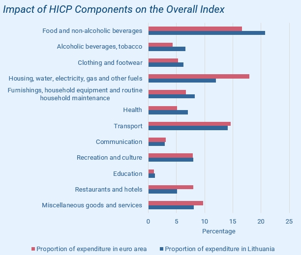
In the euro area, inflation is calculated in terms of the Harmonized Index of Consumer Prices (HICP), which tracks consumer prices in each European Union (EU) country. The specific weightings of the index components in each country are reviewed annually, based on households’ actual expenditure ratios.
Thus, the dynamics of this inflation indicator may vary for different countries due to different consumption structures. In Lithuania, food products and non-alcoholic beverages have the largest share of the basket used for calculating the HICP[2]. In the euro area, housing, water, electricity, gas, and other fuel costs generally have the highest share of expenditures.
The most used inflation indicator is the annual inflation rate, calculated as the change in the HICP for the current month compared to the same month of the previous year. This work also looks at longer-term changes and trends. The goal is to assess overall price trends rather than just short-term fluctuations due to specific components (such as energy) or individual factors (like supply chain disruptions).
Figure 1
Source – Euro area statistics
The Definition of Money Supply Is Problematic
Providing an unambiguous definition of the money supply is complex because any asset with characteristics enabling it to facilitate exchanges can be considered money. Thus, a more precise term for use in discussing the concept of money supply would be “currency”[3]. In this work, though, the concept of money will be limited to the euro, since the dynamics of price level growth relate to the ratio of specific goods and services acquired with the currency issued by the ECB.
The central bank provides three aggregate indicators to assess the money supply[4]. The money supply in a narrow sense (M1) includes banknotes, coins, and deposits that can be immediately converted into cash or used for non-cash payments. The intermediate money supply indicator (M2) includes M1 and deposits with a maturity of less than two years or that can be withdrawn with a 3-month notice. The broadest measure of money supply (M3) comprises M2 plus secondary instruments which the financial sector has brought to the market.
TABLE 2.Monetary Aggregates |
|
| M1 | Currency in circulation + Overnight deposits |
| M2 | M1 + Deposits with an agreed maturity of up to 2 years + Deposits redeemable at a period of notice of up to 3 months |
| M3 | M2 + Repurchase agreements + Money market fund (MMF) shares/units + Debt securities of up to 2 years |
This analysis will focus on M3, which is the broadest measure of money supply. It can explain the impact of a wide range of monetary policy instruments used by the ECB. The most significant component in all these measurements is still M1. That means the long-term trends in money supply changes would remain similar even when using a narrower measure.
How the Money Supply Affects Prices
Quantity Theory of Money Aims to Show Relationship Between Money Supply and Prices
One of the early scholars who formulated the Quantity Theory of Money (QTM) was the Polish astronomer, mathematician, and economist Nicolaus Copernicus.[5] The relationship between money supply and prices is also examined in the works of economists David Hume and David Ricardo, who explain inflation through the laws of supply and demand.
In the 20th century, Irving Fisher further developed the QTM, presenting it in the form of an equation of exchange, which Milton Friedman later solidified in economic research[6]. The equation aims to show that the change in prices will be equal to the product of the change in the money supply and the velocity of money divided by the level of output.
TABLE 3.Fisher’s Equation |
MV = PY |
M is the money supply; V is the velocity of money; P is the price level; Y is real output (or real GDP) |
P=MV/Y or HICP=M3*V/GDP |
Thus, assuming the velocity of money and the level of production remain constant, an increase in the quantity of money would always lead to a proportional increase in the price level.
However, several aspects of this equation need to be clarified.
First, the concept of the money supply is itself problematic. One can debate which indicator of money quantity best reflects its influence on inflation (for more about the issues of money supply, see section 1.3).
Second, the velocity of money can be calculated with the same formula, hence the equation is somewhat “circular” in nature.
And third, empirical evaluation of Fisher’s equation is problematic. Figure 2 shows the ratio of velocity times money supply (M3) to gross domestic product (GDP) alongside the annual changes in inflation in the euro area. Note that while the quantity of money was little changed during the financial crisis of 2008-2010, price deflation began only in 2011. Moreover, M3 started growing in 2019, even before the pandemic and more than a year before inflation began.
Figure 2
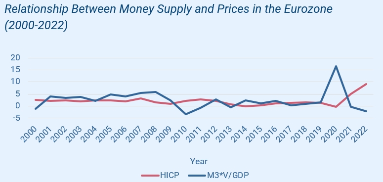
Sources: European Central Bank (ECB), Eurostat. Calculations – LFMI
The mathematical equation that expresses the QTM does not fully reveal the causal relationships between its elements. It provides a reasonably clear link between money supply and prices, but does not elaborate on the causal relationships between an increase in the quantity of money and the growth of inflation. Nor does it fully explain the differing speeds at which the effects of monetary policy manifest themselves.
The Impact of Money Demand on Price Inflation
The QTM primarily focuses on trends of money supply and only considers factors related to that. To better understand the causes of inflationary processes, the QTM needs to be supplemented with analysis of money demand. Such analysis reveals why an increase in money quantity has different effects on the price level at different times and to varying degrees.
Money demand can be understood as the total amount of money that all economic participants consider more valuable and useful than the goods and services that could be obtained with that money during a specific period. Money that is not in demand is spent by exchanging it for goods and services, which also affects the prices of other goods and services. The impact of increased money supply on prices will depend on what the recipients of the newly created money decide to do with it. If market participants choose to hoard the new cash and not spend it on goods and services, the prices of goods and services will not be affected during that specific period.
Figure 3
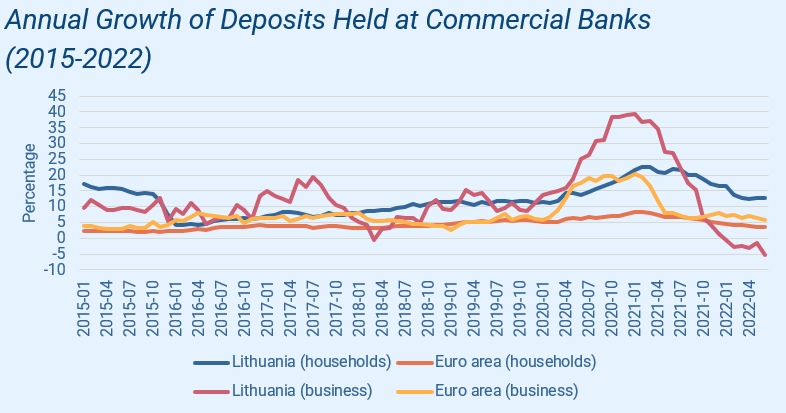
Source: Eurostat
It is the factor of money demand that can explain why different time lags occur between a rapid increase in money supply and price inflation. The impact in terms of inflation does not manifest equally quickly or to the same extent because, during a given period, economic participants may choose to save money if they value it more than the goods they can acquire with it. During financial crises or periods of uncertainty, people tend to hold more liquid assets (money), which helps protect them from potential shocks. The fact that people were inclined to save at the beginning of the pandemic is also reflected in Figure 3.
However, as the need for increased savings subsides, people start to spend the accumulated money, so the effect of the increased money supply on the prices of goods and services may take much longer to materialize.
For consumers, it is vital that money fulfil its functions as a medium of exchange, a unit of account, and a store of value.[7] Therefore, it can be concluded that the value of money, like that of any other economic good, is influenced not only by its supply but also by its demand.
Increase in Money Supply in Eurozone and Lithuania
During the Pandemic, the Quantity of Money and Inflation Increased Faster Than Usual
By examining the long-term dynamics of money supply and price levels, it is possible to explain unusual changes and anomalies in one of these variables. Figure 4 illustrates the growth of the HICP and M3 from the establishment of the euro area in 1999 until the beginning of 2022[8]. It is important to note that the money supply (with scale on the left) increased significantly faster than the price level (with scale on the right).
Figure 4
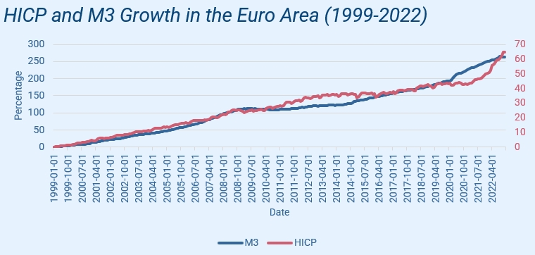
Sources: ECB, Eurostat. Calculations – LFMI
- The HICP in the euro area was 74 in 1999 and rose to 105 in 2020. In December 2022, the index reached 121. Over 23 years, the price level increased 64%. Meanwhile, during the two years of the pandemic, prices increased 15%.
- The M3 in the euro area was 4.5 trillion euros in 1999 and reached 13 trillion euros in 2020. Then within just two years of the pandemic, it increased by another quarter, reaching 16 trillion euros.
- The increase in prices in the euro area, although not as rapid as desired by the ECB, is continuous and practically uninterrupted. However, if the quantity of money remains unchanged and the prices of certain goods increase, consumers will not be able to spend as much on other goods, leading to a decrease in their prices. That would slow overall price inflation. When evaluating the dynamics of inflation, consideration is usually not given to how much prices might decrease if the quantity of money were not increased.[9]
- Therefore, it is important to assess not only the changes in the quantity of money, but also how that has changed relative to the goods produced, which are the goods that people could exchange their money for.
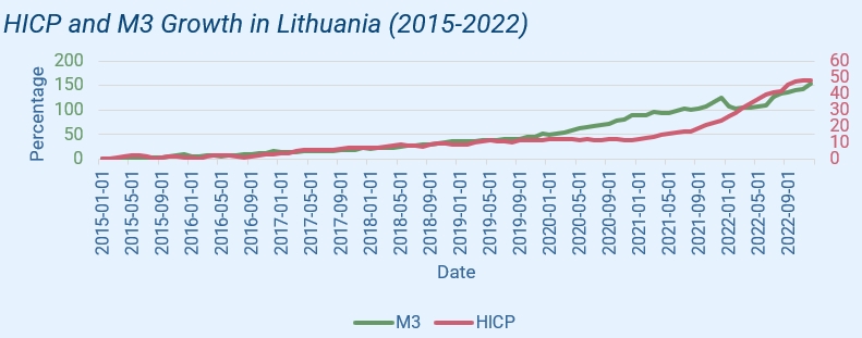
During the Pandemic, Inflation and M3 in Lithuania Increased Faster Than Usual
Figure 5
Sources: ECB, Eurostat. Calculations – LFMI
- The consumer price index in Lithuania was 99 in 2015 and had increased to 111 at the beginning of the pandemic. In December 2022, it reached 147. In short, over the period of 2015-2020 prices increased 12%, while in just 2 years of the pandemic they rose 32%.
- As regards M3 in Lithuania, it stood at 20 billion euros in 2015, increased to 31 billion euros by the beginning of 2020, and reached 42 billion euros by the start of 2022. The money supply grew 36% during the 2 years of the pandemic.
- From 2015 to 2018, M3 in Lithuania grew by 5-10% per year, while in the euro area it grew by 3-6% per year. In 2019, Lithuania increased its money supply by 10%, compared to steady growth of 5% in the euro area.
- The money supply in Lithuania grew at a faster pace during the pandemic. In 2020, M3 in the country increased 25.8%, while the eurozone average was 11.4%. In 2021, it grew a further 18.4% in Lithuania, compared to 7% growth in the eurozone.
Figure 6
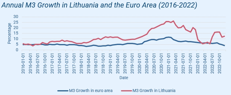
Sources: ECB, Eurostat. Calculations – LFMI
Therefore, the money supply in Lithuania grew faster than the eurozone average. This could be one factor contributing to the significantly higher price increases in Lithuania compared to the European average.
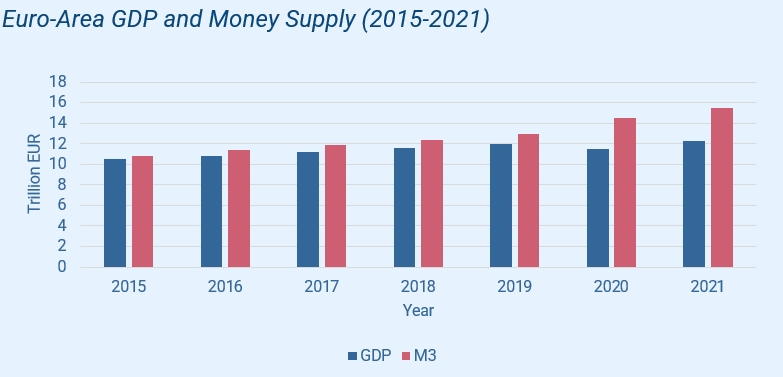
During the Pandemic, Money Supply “Diverged” from GDP
As productivity and efficiency increase, the price of goods should typically decrease. However, when the money supply grows faster than the volume of goods and services produced, the “price” of money starts to decrease, and as a result, the price of products correspondingly increases. The statistics for GDP and M3 show that the money supply grew significantly faster than the economy during the pandemic period, both in Lithuania and in the eurozone.
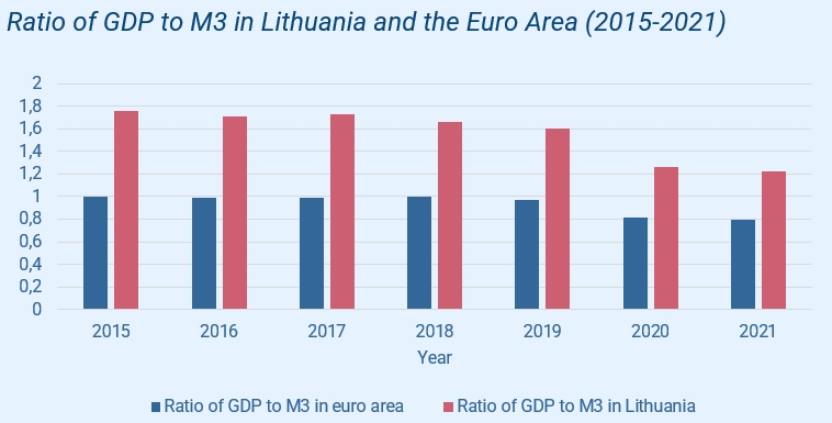
The symbolic ratio of GDP to M3 can be used to assess the portion of money in the market that is represented by goods and services.
Figure 7
Sources: ECB, Eurostat. Calculations – LFMI
- GDP in the eurozone amounted to 6.5 trillion euros in 1999, while M3 that year was 4.7 trillion euros. The two values essentially converged, at the level of 9.4 trillion euros, during the financial crisis in 2008. Since 2014, however, the money supply has exceeded the size of GDP.
- In 2019, the euro area’s GDP was estimated at 12 trillion euros, while M3 was 13 trillion euros. During the pandemic, the disparity became much bigger yet, with GDP remaining at about 12 trillion euros for 2 years, while the money supply grew to 15.47 trillion euros.
- Lithuania’s GDP was 37 billion euros in 2015 and was significantly larger than the country’s M3 money supply of 20 billion euros. The indicators kept similar proportions through 2019.
- In 2021, Lithuania’s GDP was 56 billion euros, while its money supply was 46.1 billion euros.
Figure 8
Sources: ECB, Bank of Lithuania, Eurostat. Calculations – LFMI
That means that during the pandemic growth of the money supply significantly outpaced economic growth. As a result, each euro in circulation corresponded to a decreasing share of GDP. In the history of the euro area, its economy had never had such a large money supply.
The rapid increase in the money supply relative to economic growth contributed to an increase in aggregate demand during the pandemic. Here, however, the rise in demand was due not to certain products being valued more but to the increased quantity of money. Such a situation sends a misleading signal to businesses about increased demand for their products. When prices lose their natural role of signalling to producers about demand, imbalances between supply and demand emerge, leading to periods of unsustainable economic growth and increased risks of recession.
ECB Monetary Policy Measures
Zero Interest Rates Were Not Enough to Achieve the ECB’s Inflation Target
Growth of the money supply and prices in the euro area are continuous processes. But to understand the reasons for the rapid increase in money supply during the pandemic, it is necessary to evaluate what ECB measures had the greatest impact on the M3 aggregate.
| TABLE 4 | ||
| Key ECB Interest Rates | ||
| Key ECB interest rate | Mechanism | Effect |
| Marginal lending facility | Commercial banks can borrow extra for one day by pledging sufficient assets with the central bank. This increases their liquidity. | The “price” that commercial banks would have to pay to borrow from the ECB. |
| Main refinancing operations | A weekly facility that allows financial market participants to obtain the liquidity they need. | The “price” that commercial banks have to pay to borrow from the ECB for a week. |
| Deposit facility | Allows commercial banks to hold deposits in the central bank. | The return that commercial banks can receive from the central bank by holding their reserves there. |
The ECB’s decisions related to three key interest rates which affect the euro interbank offered rate (Euribor) and are most frequently discussed in the public and media. Euribor is the interest rate at which European commercial banks are willing to lend funds to each other; it ultimately determines the borrowing costs for households and businesses.
Euribor balances between these three interest rates. Commercial banks will not be inclined to keep deposits in the central bank if other commercial banks offer higher interest rates for reserves. They will also not borrow from the central bank at the marginal interest rate if they can borrow cheaper from another commercial bank.
The size of interest rates usually affects the trends of money supply growth. The lower the cost of loans, the higher the demand for them, as more people want to obtain additional financing from commercial banks. Although the central bank does not directly increase the money supply in the market by setting the base interest rates, it does reduce or increase the demand for new loans.
- The ECB started reducing interest rates in late 2008. As the financial crisis came to an end, it attempted to increase rates in 2011 (by 25 basis points at each of two consecutive ECB meetings). However, by the end of the same year, rates were lowered again.
- The deposit rate eventually became negative in 2014, and all-time lows were reached shortly before the pandemic, in September 2019 (the deposit rate was at -0.5%, the main refinancing operations at 0.00%, and the marginal lending facility at 0.25%).
- In July 2022, when the euro area faced record-low inflation, all these rates started to increase.
Figure 9
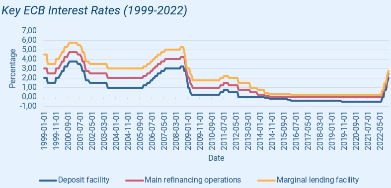
Source: ECB
Although key interest rates determine the cost at which commercial banks lend to businesses and individuals, reducing these rates does not guarantee that people will want to borrow more. The principle of diminishing marginal utility also applies to loans.
When Euribor remained artificially at 0% for a long time, the demand for cheap loans was satisfied, leading to a gradual decrease in the need for financing. This made it more challenging for the central bank, with its 2% annual inflation target, to ensure a consistent increase in the money supply solely through the regulation of key interest rates.
Significant Increase in Asset Purchase Programmes during the Pandemic
Although the key interest rates were reduced to unprecedented levels, cheap loans did not ensure economic growth in the euro area. In 2012, the Outright Monetary Transactions (OMT) mechanism was announced, allowing for the purchase of a limited amount of government bonds, but it was never actually used. The inflation rate also failed to reach the ECB’s target of 2%. Therefore, in 2014, policymakers decided to adopt new and untested measures known as quantitative easing (QE).
Through QE measures, the ECB “converts” securities held in the secondary market into new money. This increases investor liquidity, provides commercial banks with new funds. It also places financial assets such as bonds on the central bank’s balance sheet. This injection of money is more beneficial to some market participants than others, as they can use these new funds before prices have risen.
In this way, the central bank can ensure that the money supply in the economy increases as they intend. Aggregate demand is stimulated not only by expansionary financial policies but also by the direct provision of liquidity to financial asset holders. By purchasing financial assets that would otherwise have no demand, the ECB can inject money into the economy more quickly.
Furthermore, by increasing the scope of such asset purchase programmes, the central bank influences the prices of bonds, artificially increasing demand for them and thereby reducing bond yields (the difference between the price of acquiring a financial asset and the return on it over time). This means a reduction in the cost of government debt, which stimulates aggregate demand as governments are encouraged to spend relatively more. Thus monetary policy also has an impact on fiscal measures.
In 2014, the ECB began implementing an Asset Purchase Programme (APP). Policymakers resolved to use the programme “for as long as necessary to strengthen the impact of interest rates”, and to terminate it “before starting to increase the official ECB interest rates.”
Since 2014, the ECB has also implemented a series of Targeted Longer-Term Refinancing Operations (TLTRO) aimed to ensure that banks continue to lend to businesses and individuals. Under this programme, banks received funds with interest rates 50 basis points lower than the deposit facility rate on the condition that they lend these funds to the economy.
- From 2015 to 2019, securities purchases were carried out at a rate of 20-80 billion euros per year. In response to the COVID-19 pandemic, the scope of the APP was significantly expanded until the end of 2020, reaching 120 billion euros.
- Additionally, a new Pandemic Emergency Purchase Programme (PEPP) was launched. Its scale of 1.85 trillion euros was ten times larger than the APP. It was concluded in March 2022.
Figure 10
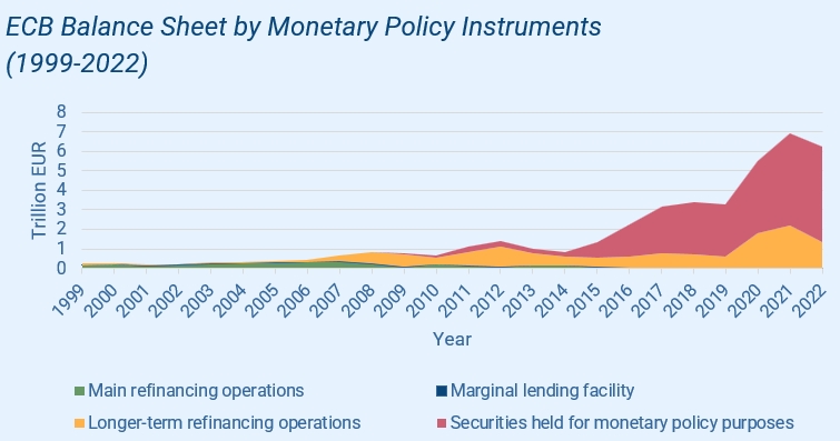
Source: ECB
Finally, in July 2022, shortly after announcing the first increase in key interest rates in eleven years, the ECB simultaneously introduced a new asset purchase instrument called the Transmission Protection Instrument (TPI) whose volumes is not limited ex-ante. However, the central bank has not yet used this measure.
Thus, it was a significant changes for the euro area when monetary policy was reoriented from traditional measures, such as interest rate regulation, to unconventional ones. Figure 10 shows how the ECB’s balance sheet steadily increased, with the greatest impact coming from the securities purchase programmes.
The ECB Now Relies More on QE than on the Regulation of Interest Rates
Analysis of the central bank’s portfolio makes it possible to assess which tools have the greatest impact on the money supply. Securities constitute the largest share of the assets held by the ECB, as shown in Figure 11. Whereas in its early stages the ECB relied primarily on key interest rates, in recent years asset purchase programmes have assumed the most weight in the arsenal of monetary policy measures.
Figure 11
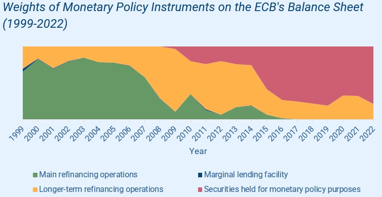
Source: ECB. Calculations: LFMI
- At first, main refinancing operations were the instrument with the most significant impact on the ECB’s balance sheet (162 billion euros). The marginal lending facility amounted to 11 billion euros and there were 75 billion euros of longer-term refinancing operations. The ECB did not hold any securities considered money policy instruments at that time.
- Before the pandemic (in 2019), purchased securities had the most weight on the ECB’s balance sheet, amounting to 2.6 trillion euros. That compared to 616 billion euros of longer-term refinancing operations.
- In 2021, longer-term refinancing operations amounted to 2.2 trillion euros, while the combined asset purchase programmes had more than twice that weight on the ECB balance sheet, at 4.7 trillion euros.
QE has become the main instrument by which the ECB conducts monetary policy. An enormous increase in M3 has been effected through securities purchases rather than by lowering interest rates. It is often noted that interest rates were reduced to near-zero levels as early as 2014, but inflation only emerged in 2022. That just strengthens the hypothesis that it was QE that had the biggest impact on the increase in the money supply rather than interest rates.
The ECB’s Impact on Lithuanian Monetary Policy
The Portfolio of Securities Purchased by the Bank of Lithuania Increased during the Pandemic
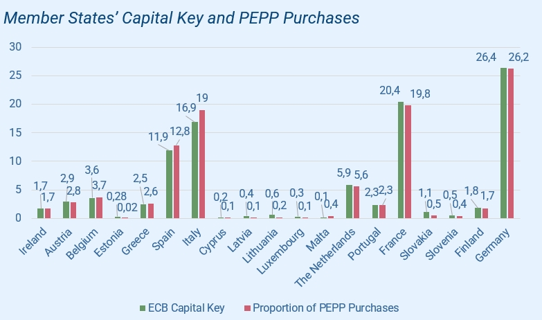
The monetary policy of the euro area is carried out by the national central banks of the member states. Policymakers envisage that QE in each member country will be guided by the “capital key”. That contribution of each national central bank to the ECB is calculated based on the country’s share of the GDP and the population of the European Union. Purchases of securities within the jurisdiction of each national central bank are made in accordance with these proportions.
It is worth noting that the capital key is more a limit than an obligation to conduct a specific share of QE. National central banks are not required to exhaust it fully. The amount of bonds purchased by a national central bank also depends on the decisions of that country’s government to increase or decrease its budget deficit.
- As of December 2021, the capital key for Lithuania was set at 0.58. By comparison, Latvia’s was 0.39 and Estonia’s 0.23. This figure is reviewed at least once every 5 years.
- At the end of 2015, the first year of euro adoption, securities held by the Bank of Lithuania for monetary policy purposes totalled 2.5 billion euros. By the end of 2019, the amount had quadrupled to 10.5 billion euros.
- During the pandemic period, the Bank of Lithuania’s securities portfolio grew by more than 2 billion euros, reaching 13 billion euros in 2021.
In implementing the PEPP, the member states generally adhered to the framework of the capital key, with a few minor exceptions. Estonia stands out in this context, as its purchases were significantly lower than allowed by the capital key (only 0.02% of the total eligible amount). Lithuania and Latvia also bought less than they could have.
The Money Supply in Lithuania Grew Faster as It Was Proportionally Smaller Than in the Euro Area
Figure 12
Source: ECB. Calculations: LFMI
M3 in all three Baltic countries grew faster than the eurozone average. In 2022, Lithuania’s GDP was still larger than M3, while in the eurozone, the opposite was true – M3 was larger than GDP (see section 3.3). This means the rate of M3 growth may depend not only on the decisions of the national central bank but also on the comparative base and the overall eurozone policy, as ECB decisions to increase the money supply affect the entire euro system.
When the money supply is increased based on GDP proportions, it grows faster in countries where it is relatively smaller at the time. Thus, implementing monetary policy according to the capital key rule may result in a faster increase in the money supply in those countries where M3 has been relatively minor.
Conclusion
- Price levels are influenced not only by increases in the money supply but also by money demand. The impact of an increase in the money supply on prices depends on how people choose to use the “new” money.
- A choice to save money rather than spend it was seen at the beginning of the pandemic. Due to uncertainty and limited consumption opportunities, individuals and economic entities saved more. Therefore, the increase in money supply did not immediately lead to price inflation.
- Prices have risen steadily ever since the creation of the euro area. During the pandemic, however, the expansion of the money supply significantly exceeded the growth rate of production and services, creating conditions for a significant increase in price levels.
- Even by reducing the key interest rates to zero, the ECB was unable to ensure a stable increase in the money supply. Therefore, since 2014, the ECB has implemented asset purchase programmes. The volumes of such purchases significantly increased during the pandemic. This allowed the ECB to achieve an increase of the money supply in the euro area by a quarter over the 2 years of the pandemic.
Ergo, although price inflation is influenced by various factors, this analysis shows that the ECB’s expansionary monetary policy resulted in a significantly faster increase in the money supply during the pandemic. The constrained economy was not able to grow in such a fast pace, so M3 diverged from GDP. This created conditions for general inflation, not only growth of prices in a few specific segments.
Expansive monetary policy during the pandemic helped to mitigate the potential consequences of an economic contraction and stimulated aggregate demand. The side effect of these ECB actions became visible after a time lag, as is typical with monetary policy. Since the money supply grew significantly faster than volumes of goods and services, prices started to rise sharply. Under such circumstances, money may not effectively perform its inherent functions as a medium of exchange, store of value, and unit of account. Inflation after the pandemic simply demonstrated that sooner or later society must pay the “price” for cheap money.
[1] Sigitas Šiaudinis, „Komentaras: Kodėl centriniai bankai, siekdami mažos infliacijos tikslo, nebereguliuoja pinigų kiekio“, 2023, p. 6.
[2] Euro area statistics, “How Is Inflation Measured?”, at https://www.euro–area–statistics.org/digital–publication/statistics–insights–inflation/bloc–2a.html.
[3] Friedrich A. Hayek, “Denationalisation of Money”, The Institute of Economic Affairs, London, 2007, p. 56.
[4] ECB, “The ECB’s Definition of Euro Area Monetary Aggregates”, at https://www.ecb.europa.eu/stats/money_credit_banking/monetary_aggregates/html/hist_content.en.html.
[5] Mises Institute, “Copernicus and the Quantity Theory of Money”, https://mises.org/library/copernicus–and–quantity–theory–money.
[6] Milton Friedman, “The Quantity Theory of Money: A Restatement”, in Studies in Quantity Theory of Money, Chicago: University of Chicago Press, 1956.
[7] Phillip Bagus, “The quality of money”, Quarterly Journal of Austrian Economics, Vol. 12, No. 4, 2009, p. 23.
[8] The countries that joined the euro area after 1999 accounted for less than 4% of the total M3 of the euro area in 2022. Greece joined the euro area in 2001, Slovenia in 2007, Cyprus and Malta in 2008, Slovakia in 2009, Estonia in 2011, Latvia in 2014 and Lithuania in 2015. Thus the accession of these countries had only a marginal impact on the dynamics of the money supply.
[9] Roland Baader, “Money-socialism”, LFMI, p. 38.
Continue exploring:
Impacts of the Russian War in Ukraine on CEE: 4liberty.eu Review No. 19 Now Available Online