
Economic time series exhibit periodically recurrent movements at the daily, weekly, and monthly levels. Also known as seasonality, it has been usually treated as a nuisance to be removed prior to analysis. Often, data is already deseasonalised by data providers since it distracts from medium-term time trends and long-term cycles.
Moreover, seasonality disappears when data are aggregated to a yearly basis – it is a phenomenon at work at shorter time frames. It is an expression of the cyclical nature of much of human activity. For example, most workers do not work on weekends, days off work tend to cluster around public holidays, and income is usually received on a fixed day of month.
Therefore, sudden changes in seasonality can be interpreted as a measure of economic disruption. Using a state-space framework of time series analysis (wherein seasonality is modelled as time-varying, and estimated using the Kalman filter), this paper analyses the changes in seasonality brought about by the coronavirus pandemic of 2020. While no significant crisis effects appear in daily euro-denominated transfers from Slovenia to Bosnia and Herzegovina, trend levels in Slovenian aggregate electricity consumption did decline noticeably.
The day-of-the-week patterns remained stable even in times of the lockdown. Not so in Apple mobility data, where seasonality is shown to have altered significantly in Slovenia but also in Sweden, Serbia, Romania, Germany, and Austria.
Introduction
“Seasonality means special annual dependence. Many weekly, monthly, or quarterly economic time series exhibit seasonality” (Sargent 2001). It is a property that can be only detectede when data is measured more than just once a year.
In fact, seasonality is meant to cancel out when high-frequency data is aggregated to lower frequencies. This, in turn, usually means that seasonal effects are constrained to sum up to zero if assumed additive (Hyndman et al. 2008, 123).
In times of crisis, seasonality can be expected both to change and reassert itself. It can no longer be ignored. After all, seasonality is one way the predictable economic activity rhythm is reflected in economic data. It captures the effects of recurring monthly deadlines, annual vacations, bank holidays, and the seasons of nature.
If economic activity is disrupted, so are the seasonal patterns in economic data. Conversely, changes in seasonality can be used as a quantitative measure of how a crisis disrupts the daily workings of an economy. Indeed, seasonality was found to have profoundly altered during the Great Recession, reflecting the shattered economic lives of the many (Wright 2013).
Has seasonality been changing during the pandemic of 2020? This article aims to collect stylised facts about the disruptions in seasonal patterns at the weekly level. This is the time scale where disruption to daily life, the basic rhythm of economic activity, should manifest itself. Also, it is the only time frame where seasonal patterns can be reliably identified even few months into an ongoing pandemic.
For Slovenia, at least three data sources are sufficiently granular to identify day-of-the-week effects in real time: (1) money transfers to high-risk countries, (2) electricity use, and (3) Apple mobility data. The latter also allows for international comparisons. To keep the analysis tractable, five European countries represent markedly different trajectories: Sweden, Serbia, Romania, Germany, and Austria.
Using seasonality as a measure of economic (dis)order is conceptually not new. The stylised fact that seasonality appears more pronounced in 19th-century macroeconomic datasets than 20th-century ones has been long interpreted as an indicator of economic progress. “The loss of seasonality, the separation of credit flows from natural rhythms, and a totally socially constructed reality might be seen by some as indications of economic development and the progress of human civilization” (Klein 1997, 118).
What follows is a short review of the main approaches to seasonality taken in economics (Section 1). In a nutshell, there are three of them (Subsection 1.1). Daily seasonality raises further issues (Section 2). The statistical significance of seasonal effects is explored in a state-space structural framework, which is then adopted throughout the article (Subsection 2.1).
Two case studies drawn from Slovenia demonstrate that seasonality should be treated neither as given nor as necessarily time-varying (Subsection 2.2). However, seasonal effects in daily mobility data are both significant and dynamically changing (Section 3). This is inferred within a multivariate setting (Subsection 3.1), with particular attention given to lower-frequency patterns that remain beyond full identification for data reasons (Subsection 3.2). Later, stylised facts are collected (Subsection 3.3).
1 Seasonality in Economics
Most studies that explicitly address seasonality tend to look at either (1) month-of-the-year effects (that is, seasonal patterns appearing at lag 12 in monthly data) or at (2) quarterly effects (at lag 4 in quarterly data). Researchers have documented stably recurring patterns in several different time series, sometimes even arguing that one variable is a cause for another based on a similar seasonality structure of the two.
Lam and Miron (1991) illustrate both the abundance of seasonal data, and the conundrum seasonality can create for causal interpretation. For example, they find “that births are highly seasonal in all human populations, even for very recent periods in highly industrialized low-fertility populations. The timing of the seasonal patterns, however, differs widely across populations.”
Traditionally, these patterns have been linked to other series with pronounced monthly seasonality.
Therefore, Lam and Miron consider weather data such as air temperature, labour force participation, the agricultural harvest cycle, the number of marriages, and the distribution of holidays throughout the year. Nonetheless, none of these patterns provides a consistent explanation for the significant yet country-specific monthly seasonality in births.
This list of seasonal variables is by no means exhaustive. Text-book examples of monthly seasonality include industrial production, retail sales of clothing, and retail credit, while both daily and monthly patterns can be found in the S&P500 stock index (Ghysels and Osborn 2001).
Also, seasonality “is one of the most remarkable features of tourism. It is a global phenomenon that affects the vast majority of tourist destinations.” Vergori (2016).
1.1 Three Approaches to Seasonality
“Seasonality has been a major research area in economics for several decades,” summarise Brendstrup et al. (2004). They identify three interrelated groups of economic approaches to seasonality. “The first group, pure noise model, consists of methods based on the view that seasonality is noise contaminating the data or, more correctly, contaminating the information of interest for the economists.
The second group, time-series models, treats seasonality as a more integrated part of the modeling strategy, with the choice of model being data driven. The third group, economic models of seasonality, introduces economic theory, that is, optimizing behavior into the modeling of seasonality.”
In recent years, the tide has been turning against the first group. Seasonality is increasingly seen in economics as “an integral part of the modeling process, and where there is an increased awareness that use of seasonally adjusted data very easily leads to errors and in addition throws away valuable information” (Brendstrup et al. 2004).
In fact, substantive economic insights can gleam from seasonality. For instance, “the observed seasonality of box-office revenues has been found to reflect both seasonality in underlying demand for movies and seasonality in the number and quality of available movies” (Einav 2007).
It is not only the possibility of economic interpretation that speaks in favour of explicit models of seasonality. The existing approaches used by statistical authorities around the world have repeatedly been found wanting.
Crucially, they fail to remove the seasonal patterns completely – some seasonal variation can remain even after the supposed deseasonalisation. Since economic data are widely used in decision-making, this is more than an academic concern. If no patterns are expected and yet continue to exist, bad decisions are likely to be made.
“This phenomenon, called residual seasonality, makes it difficult for policymakers to know whether a weak first quarter is due to an actual downturn or an understated number” (Owyang and Shell 2018). For US GDP data, the “size of this residual seasonality is economically meaningful and has the ability to change the interpretation of recent economic activity” (Lunsford 2017).
2 Conceptual Issues with Daily Seasonality
To identify inter-day patterns, the minimum requirement is having data spaced at daily or even finer intervals. This severely limits the scope of available data sources – publicly available macroeconomic series are only rarely reported at such granularity. Also, daily data is a necessary but not a sufficient condition. Not all daily data exhibit stable patterns at lag 7.
In other words, seasonality is not necessarily an artifact of statistical analysis, even though inappropriate modelling has been shown to generate spurious seasonality (cf. Franses et al. 1995). Just because an economic variable is measured every day, it does not necessarily display day-of-the-week patterns.
Moreover, there is no inherent reason why seasonality, when it exists, should always vary with time. For some series, the time variance of seasonality is indeed negligible, and the data generating process can be much more parsimoniously modelled with a fixed, deterministic formulation.
These points can be illustrated with two daily time series covering the period from 1 January 2018 to 31 May 2020: (1) euro-denominated money transfers from Slovenia to Bosnia and Herzegovina (Office for Money Laundering Prevention 2020), and (2) Slovenia-wide electricity usage measured in megawatts (MW) (Eles 2020).
Note that both series are constructed from public sources, i.e., they were not reported as a daily series to begin with (the first is compiled from a list of time-stamped transactions, the second is aggregated from hourly data). There appear to be no significant Covid19-related changes in either’s seasonality.
In the first example, it is because there is no daily seasonality to speak of. In the second example, fixed daily seasonality remains the favoured formulation even when the sample includes the pandemic.
2.1 The Testing Set-Up
To reach these conclusions, both variables are investigated univariately, using structural state-space systems of equations estimated with the Kalman filter (Harvey 1989, Durbin and Koopman 2012). Each time series is transformed to natural logarithms and decomposed into its structural components:
= + + +∑ ,, =1 + , ∼ (0, 2 ), = 1, … , , (1)
so that is the trend, is the seasonal, is the cycle, and the irregular. Dummy variables identifying calendar effects and bank holidays are while are corresponding unknown regression coefficients. The list of work-free days is sourced from the Slovenian government (Ministry of Public Administration 2020).
The notation means the irregular component is normally and independently distributed with mean zero and variance . In other words, it is a Gaussian disturbance, and it is different from disturbances affecting other structural components. All disturbances are mutually independent. The trend can be time varying.
The money transfer series is modelled with the local linear trend specification:
= −1 + −1 + , ∼ (0, 2 ), (2) = −1 + , ∼ (0, 2 ), (3)
For electricity usage, the trend is described using the simpler local level model – the slope terms and the stochastic slope disturbance are omitted so that the specification simplifies to a random walk with noise. Since there is an odd number of days in a week (the number of seasonal frequencies for electricity data and 5 for transactions), the seasonal component is modelled as
= ∑ , , −1 2 =1 (4)
where each , is given as
[ , , ∗ ] = [ cos sin −sin cos ][ ,−1 ,−1 ∗ ] + [ , , ∗ ], = 1, … , − 1 2 , = 1, … , , (5)
where = 2⁄ stands for the frequency (in radians) while , and , ∗are two mutually independent Gaussian white noise disturbances with zero means and common variance 2 . Similarly, the cyclical component is
[ ∗ ] = [ cos sin −sin cos ]
[ −1 −1 ∗ ] + [ ∗ ], = 1, … , , (6)
2.2 Seasonality Test Results
Considering the money transfer data (Figure 1), the formal statistical test for the significance of seasonality components is performed on the final state vector. The value of the seasonal χ² test is 1.71 (corresponding to a probability of 0.788), implying the seasonal pattern is so weak to be practically indistinguishable from zero.
Moreover, there is no individual single day-of-the-week effect that comes even the hurdle of statistical significance, let alone passing it (the estimated probabilities range from 0.289 to 0.685).
Figure 1: Euro-denominated transfers from Slovenia to Bosnia and Herzegovina between 1 January 2018 and 31 May 2020
 Source: Office for Money Laundering Prevention 2020 and own calculations.
In the electricity usage series, in contrast, seasonality is highly statistically significant throughout the estimation sample (Figure 2). The value of the seasonal χ² test is 4716.00 (corresponding to a probability of 0.000). However, seasonality is also revealed to be fixed, that is, deterministic – the variance of seasonal disturbances is estimated at 0.000.
Figure 2: Electricity usage in Slovenia between 1 January 2018 and 31 May 2020, trend level and seasonal components
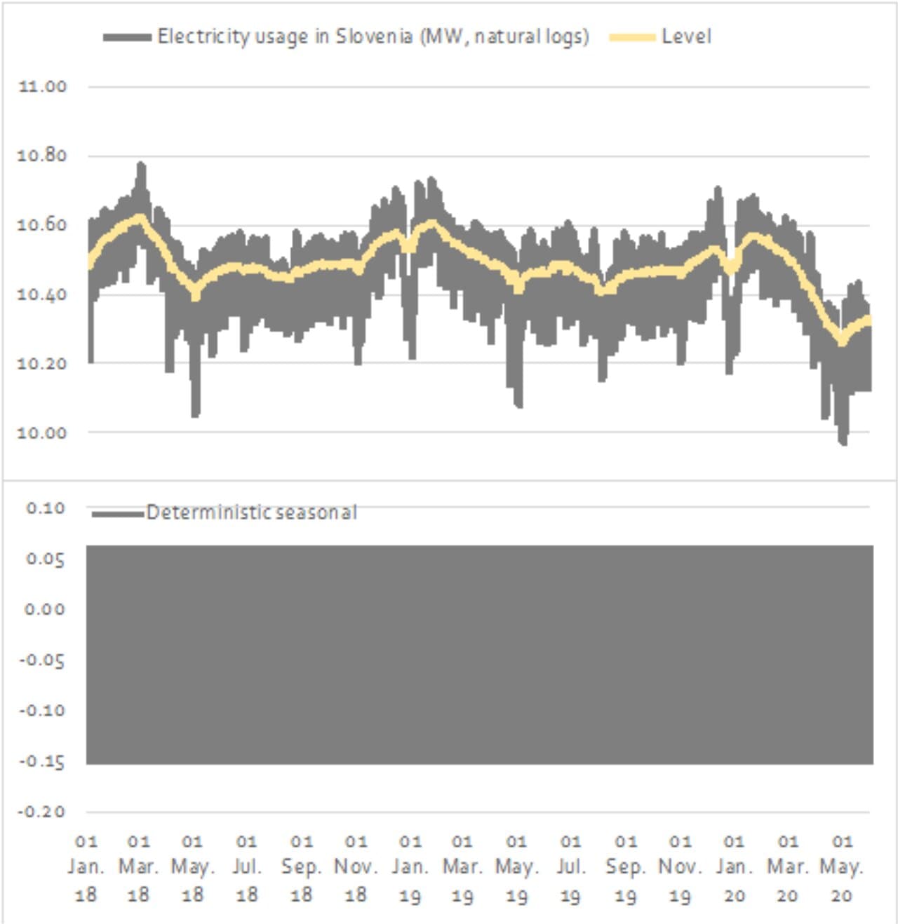 Source: Eles 2020 and own calculations.
These results not only introduce the state space approach, which is also used in sections bellow. They also provide reassurance that this methodology is indeed able to differentiate between time-varying, fixed, and non-existent seasonality. The stylised facts uncovered using this type of procedure are not spurious.
Also, the trend in electricity usage experienced a clear and significant downturn in spring 2020. What pandemic did not do, however, is to alter the seasonal patterns, indicating that the largest electricity consumers, despite decreasing consumption, kept the same consumption schedule.
3 Changes in Mobility
Since seasonality reflects basic patterns of everyday life, it should be perhaps expected that the lives of ordinary consumers are more disrupted by the pandemic than the schedules of heavy industrial electricity users. Mobility data is especially well-suited to capture such an effect on society at large.
Considered through the lens of movement, the daily human life consists of long stretches of relative immobility interspersed with bursts of intensive activity. The morning commute from home to the workspace and then back home again, perhaps with further movement in the afternoon related to leisure activities, generates seasonal patterns.
This section looks at how this daily rhythm was disrupted in 2020, comparing changes in Slovenian mobility with those in Sweden, Serbia, Romania, Germany, and Austria.
To aid the monitoring of 2020 epidemiological containment efforts against Covid-19, the two dominant providers of smartphone operating systems (iOS and Android) decided to publish anonymised data on the mobility of their phone users globally (Apple 2020, Google 2020). While Apple data is based on the volume of direction requests in Apple Maps, Google tracks smartphone location data. Both corporations report rescaled data, that is, values divided by a baseline.
However, its particular form of normalisation renders Google’s data less appropriate for modelling day-of-the-week effects. Namely, Apple uses a single day, the 13 January 2020, as its benchmark.
In contrast, Google divides by the median value of the same day of the week during the 3 January – 6 February 2020 five-week period, which can be thought of as a simple form of seasonal adjustment. This is why Apple data is preferred for seasonal analysis, even though it is relatively less precise.
3.1 The Statistical Model
First, we relax the assumption that drivers and walkers are each facing mutually independent shocks – despite living in the same country and experiencing the same Covid-19 containment measures. In other words, shocks can correlate across different mobility series within a given country. This can be achieved with a system of seemingly unrelated time series equations (SUTSE). Rather than analysing each time series in isolation, each with its own univariate system of state and measurement equations, both series for each country are stacked into a vector and analysed simultaneously (Harvey 1989, Durbin and Koopman 2012):
= + + +∑ ,, =1 + , ∼ (, 2 ), = 1, … , , (7)
Figure 3 illustrates the results of this decomposition on Slovenian mobility time series.
Figure 3: State-space decomposition of Slovenian mobility series
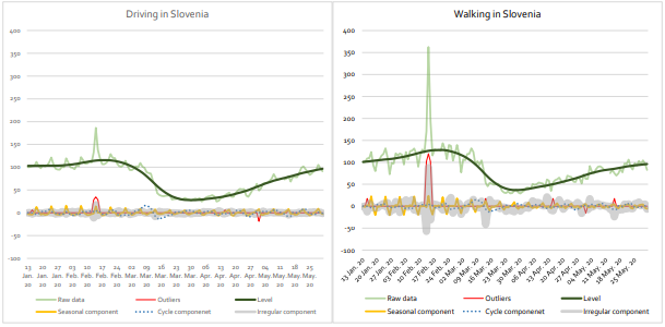 Note: Data is normalised to 100 (13 January 2020 being the benchmark). Components are in % points.
Source: Apple 2020 and own calculations.
Since Apple reports figures rescaled relative to the 13 January benchmark, data is analysed directly in levels (that is, in contrast with the money transfer and electricity usage series, it is not log-transformed). The model-set up mirrors the univariate case (Equations 1–6) except that (notice the bold notation) is now a vector of N × 1 observations.
The same holds for other unobserved components. Stochastic disturbances are vectors with N × N variance matrices. Given the short sample size, it is particularly important to avoid overfitting. Therefore, the smooth trend specification is chosen:
= −1 + −1, (8) = −1 + , ∼ (, 2 ), (9)
As for the cycle, the damping factor and frequency are the same for both series in each system (that is, fixed by country), where and are N × 1 vectors:
[ ∗ ] = { [ cos sin −sin cos ] ⨂}[ −1 −1 ∗ ] + [ ∗ ], [ ∗ ] = 2 ⊗ (10)
3.2 Approaching Seasonality at Other Frequencies
Why the cycle and the dummy variables? Since Apple mobility starts with 13 January 2020, day-of-the-week effects are the only type of seasonality that can be estimated reliably. Unfortunately, it is far from being the only one. Banking holidays also form a recurring annual pattern. Another source of monthly spikes in activity are various bureaucratic deadlines that tend to cluster around the first or the 15th day of the month, effectively doubling the number of seasons to 24. At the monthly level, mobility should reflect natural seasonal variation in weather. For example, spring is more conducive to taking walks than winter. Clearly, the sample provides only single realisations of recurrent processes operating at lower frequencies. This is much less than the theoretical minimum required for a simple exponential smoothing model of monthly seasonality – 17 months’ worth of data points, which itself might not be enough to “deal with randomness in the data” (Hyndman and Kostenko 2007).
In the structural state-space approach to time series decomposition, it is possible to partly recover such month-of-the-year effects by extending the model with a stochastic cycle and a set of dummy regressors (set 1 on the date of a bank holiday and 0 otherwise). Table 1 summarises the lower-frequency seasonality terms in mobility models. The estimated cycle can be as short as two weeks in Germany (implying that significant deadlines occur twice a month), or longer than in a month in Austria and Serbia. During the first wave of the 2020 pandemic, Easter failed to significantly affect mobility patterns in Austria and Slovenia.
Table 1: Recovering annual patterns from a few months’ data (13 January – 31 May 2020)
| Period of the cycle (in days) | Significant day-of-the-month dummies | Significant holiday dummies (outliers) | |
| Austria |
33 |
– | – |
| Germany |
14 |
– | Driving: St. Valentineʼs, Easter, May Day |
| Romania |
22 |
Driving: the 15th day of the month (or the last working day preceding the 15th if the latter happens to be work-free). |
Driving: Orthodox Easter, May Day |
| Serbia |
37 |
Driving: the 1st day of the month, the 15th day (or the last working day preceding the 15th if the latter happens to be work-free). | Driving and walking: Orthodox Easter, May Day. |
| Slovenia |
20 |
Driving and walking: the 15th day of the month (or the last working day preceding the 15th if the latter happens to be work-free). | Driving and walking: St. Valentineʼs (coinciding with the start of the winter school break in the Western half of the country).Driving: May Day. |
| Sweden |
27 |
– | Driving and walking: Easter, May Day. |
3.3 Lessons in mobility
The estimated smooth trends are shown in Figure 4. Such visualisations are the suggested way to inspect mobility series – “Day of week effects are important to normalize as you use this data” (Apple 2020). In other words, seasonality and other presumed noise are to be filtered away to reveal long-term tendencies.
Figure 3: Estimated trends in Apple mobility series
 Note: Data is normalised to 100 (13 January 2020 being the benchmark). Levels are measured in % points.
In early March 2020, mobility trends declined precipitously across the entire sample, both in driving and walking. By early April, the tide had again turned and in late May, many countries already exceeded pre-crisis levels.
Also, the recovery in mobility levels appears to be much quicker in driving data than in walking. The asymmetrical impact of the Covid-19 crisis on the two modes of personal mobility is even more pronounced in the seasonal components.
In Figure 5, weekly patterns in mobility are displayed overlaid for each country. In general, walking used to exhibit significant weekly variation before the pandemic. Except for Serbia, walking was by far the more seasonal activity compared to driving. During the first wave of the pandemic, both series started to exhibit similarly subdued patterns.
Moreover, the changes in seasonality are slower to revert to pre-crisis levels than those in the slope of the trend level. By late May, mobility trends might have returned to their winter peaks but still, they displayed weekly patterns remarkably alike those at the height of the epidemic.
Figure 4: Estimated seasonality in Apple mobility series
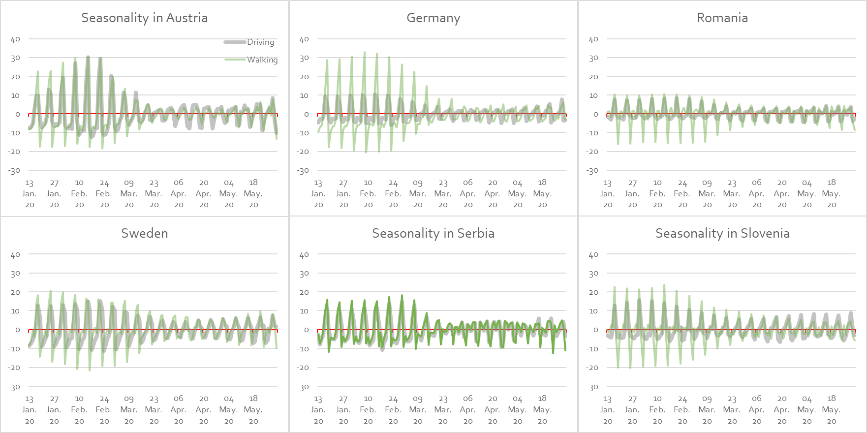 Note: Day-of-the-week effects are expressed as % point deviations from the trend level.
The results of the seasonal decomposition are further explored in Table 2. Daily effects are compared over two periods, namely the first and the last week in the time sample. In the course of 2020, seasonal variation decreased markedly. The most pronounced form of seasonal disruption appears when the seasonal component switched signs.
For example, Thursday used to lie slightly below the weekly average for driving in Slovenia. In late May, it was one of the most popular days for driving. Two observations stand out: (1) most sign changes affect Thursday effects, and (2) no such flips occurred on Friday. Which remains one of the most popular days for both driving and walking.
Table 2: Estimated day-of-the-week effects (% points)
|
Monday |
Tuesday |
Wednesday |
Thursday |
Friday |
Saturday |
Sunday |
|||||||||
|
13–19 Jan. 2020 |
25–31 May 2020 |
13–19 Jan. 2020 |
25–31 May 2020 |
13–19 Jan. 2020 |
25–31 May 2020 |
13–19 Jan. 2020 |
25–31 May 2020 |
13–19 Jan. 2020 |
25–31 May 2020 |
13–19 Jan. 2020 |
25–31 May 2020 |
13–19 Jan. 2020 |
25–31 May 2020 |
||
|
Driving |
Austria |
-8 |
0 |
-7 |
1 |
-5 |
3 |
3 |
2 |
10 |
8 |
10 |
-3 |
-3 |
-10 |
| Germany |
-5 |
-1 |
-3 |
-1 |
-3 |
1 |
-2 |
0 |
9 |
8 |
5 |
-3 |
-2 |
-3 |
|
| Romania |
-1 |
1 |
-2 |
0 |
-3 |
-1 |
1 |
2 |
8 |
4 |
0 |
-4 |
-2 |
-3 |
|
| Serbia |
-3 |
0 |
-8 |
-3 |
-4 |
-1 |
-3 |
0 |
8 |
4 |
11 |
4 |
0 |
-3 |
|
| Slovenia |
-3 |
-6 |
-4 |
-4 |
-4 |
0 |
0 |
3 |
13 |
9 |
3 |
0 |
-4 |
-3 |
|
| Sweden |
-9 |
-7 |
-7 |
-6 |
-5 |
0 |
-3 |
2 |
4 |
7 |
13 |
2 |
7 |
2 |
|
|
Walking |
Austria |
-8 |
-1 |
-8 |
1 |
-5 |
4 |
2 |
-1 |
15 |
8 |
23 |
2 |
-17 |
-13 |
| Germany |
-9 |
-4 |
-7 |
-2 |
-6 |
-3 |
-2 |
2 |
14 |
5 |
29 |
6 |
-18 |
-3 |
|
| Romania |
1 |
4 |
1 |
1 |
-2 |
2 |
1 |
2 |
10 |
3 |
4 |
-5 |
-16 |
-9 |
|
| Serbia |
-2 |
2 |
-7 |
-1 |
-5 |
1 |
0 |
3 |
11 |
5 |
16 |
2 |
-12 |
-11 |
|
| Slovenia |
0 |
2 |
-2 |
-3 |
2 |
2 |
1 |
4 |
23 |
4 |
-4 |
-4 |
-20 |
-6 |
|
| Sweden |
-8 |
-2 |
-6 |
1 |
0 |
-2 |
-4 |
1 |
14 |
8 |
18 |
3 |
-14 |
-10 |
|
Note: Number pairs where the seasonal effect switched signs during 2020 are shown in bold.
4. Conclusion
The Convid-19 pandemic of 2020 severely unsettled the daily life of nations, which is reflected in the changing seasonal pattern across several variables for Slovenia and five other European countries. However, the impact is far from uniform.
No significant changes can be detected in money transfers. In data on electricity usage, Covid-19 affects the trend but leaves seasonality alone. Both trend levels and seasonal effects change in Apple mobility data.
Moreover, these disruptions turned out to be far more persistent in the seasonal components compared to the trend components, where mobility can already be seen exceeding pre-crisis levels.
In terms of the changes in weekly patterns, Thursday effects have reversed signs in almost all countries in the sample, across both modes of mobility. In contrast, no such flips occurred on Friday, which remains one of the most popular days for both driving and walking.
References
Apple. 2020. Mobility trends reports. Accessed 5 June. https://www.apple.com/covid19/mobility.
Brendstrup, Bjarne et al. 2004. “Seasonality in economic models.” Macroeconomic Dynamics, 8: 362–394.
Durbin, J. and S. J. Koopman. Time series analysis by state space methods, 2nd edition. Oxford: Oxford University Press.
Einav, Liran. 2007. “Seasonality in the U.S. motion picture industry.” RAND Journal of Economics 38 (1): 127–145.
Eles [Slovenian power transmission system operator]. 2020. Electricity usage data. Accessed 5 June. https://www.eles.si/trzni-podatki.
Franses, Philip Hans, Svend Hylleberg and Hahn S. Lee. 1995. “Spurious deterministic seasonality.” Economics Letters 48: 249–256.
Ghysels, Eric, and Denise R. Osborn. 2001. The econometric analysis of seasonal time series. Cambridge: Cambridge University Press.
Google. 2020. Covid-19 community mobility reports CSV documentation. Accessed 5 June. https://www.google.com/covid19/mobility/data_documentation.html?hl=en.
Harvey, Andrew C. 1989. Forecasting, structural time series models and the Kalman filter. Cambridge: Cambridge University Press.
Hyndman, Rob J. and Andrey V. Kostenko. 2007. “Minimum sample size requirements for seasonal forecasting models.” Foresight 6: 12–15.
Hyndman, Rob J. et al. 2008. Forecasting with Exponential Smoothing: The State Space Approach. Berlin: Springer.
Klein, Judy L. 1997. Statistical Visions in Time: A History of Time Series Analysis 1662–1938. Cambridge: Cambridge University Press.
Lam, David A. and Jeffrey A. Miron. 1991. “Seasonality of births in human populations.” Biodemography and Social Biology 38 (1–2): 51–78.
Lunsford, Kurt G. 2017. “Lingering Residual Seasonality in GDP Growth.” Federal Reserve Bank of Cleveland Economic Commentary 2017-06.
Ministry of Public Administration. 2020. Seznam praznikov in dela prostih dni v Republiki Sloveniji [List of holidays and work-free days in Slovenia]. Accessed 5 June. https://podatki.gov.si/dataset/seznam-praznikov-in-dela-prostih-dni-v-republiki-sloveniji.
Office for Money Laundering Prevention. 2020. Nakazila v tvegane države [Money transfers to high-risk countries]. Accessed 5 June. https://www.gov.si/drzavni-organi/organi-v-sestavi/urad-za-preprecevanje-pranja-denarja/o-uradu-za-preprecevanje-pranja-denarja/sektor-za-sumljive-transakcije/.
Owyang, Michael T. and Hannah G. Shell. 2018. “Dealing with the Leftovers: Residual Seasonality in GDP.” Federal Reserve bank of St. Louis Regional Economist Q4.
Sargent, Thomas J. 2001. Foreword to The econometric analysis of seasonal time series, by Eric Ghysels and Denise R. Osborn, xiii–xiv. Cambridge: Cambridge University Press.
Wright, Jonathan H. 2013. “Unseasonal Seasonals?” Brookings Papers on Economic Activity Fall: 65–126.
The paper was published in The Visio Journal No. 5.
The article was originally published at: http://visio-institut.org/pandemic-disruptions-in-economic-seasonality.
Continue exploring:
Life After Lockdown: What Will the World Look Like After Coronavirus Pandemic?
COVID-19 Pandemic and Its Immediate Impact On Ukrainian Economy